Twenty Step Workflow

• Completion success depends upon accurate parameters determined from petrophysical analysis.
• Many stimulation designs are faulty because of poor quality sonic and density data.
• Raw log data are often inadequate due to rough borehole conditions and light hydrocarbon effect.
  • Stimulation design software expects data for the water filled case.
• In some unconventional reservoirs, the presence of organic matter confounds standard log analysis models.
  • Organic matter looks a lot like porosity to most porosity-indicating logs.
  • A single log, or any combination of them, will give highly optimistic porosity and free-gas or oil saturations.
    • an organic matter correction is required
• This workflow explains how to deal with poor quality sonic and density data, for the purpose of calculating mechanical rock properties, for input to hydraulic frac software modeling packages (GOHFER, FRACPRO and MFrac).
• Complications tied to organic rich reservoirs are also examined. The shale and organic matter corrected model is presented as a solution.

• LAS (Log ASCII Standard) files must be reviewed.
  • curve availability
  • define type (key) wells
• A three well minimum is recommended for projects.
  • Rarely will the subject well have all required data needed to complete a calibrated petrophysical analysis.
  • Offset wells should always be reviewed and used to put together the best data set possible.
  • The accuracy of the petrophysical model improves with an increased number of wells reviewed.
• A cored well should always be included (if possible).
• A text editor (Notepad, Wordpad) can be used to open LAS files to review curve data and borehole parameters.
• Measured depth logs should always be loaded, along with a deviation survey.
  • allows reference between MD, TVD, and TVDSS

• Logs must be checked for depth control.
  • an expanded depth plot track is very useful for this
• Matrix porosity scales must match (quartz, calcite or dolomite).
• Units must be consistent for all logs being run.
• Logs may need to be normalized before being run.
• NULL values and spikes over short intervals need to be fixed.

• Caliper and density correction logs are used to identify borehole intervals which are washed out (larger diameter than the drill bit).
  • calculation sequence may need to be modified over these intervals
  • reconstructed logs are often required

• Petrophysicists define volume shale as the bulk volume of the rock composed of clay minerals and clay bound water.
• Gamma ray log is typically used to calculate shale volume.
  • A non-linear relationship between shale and clean endpoints is required for radioactive intervals (Clavier, etc.).
• A spectral gamma ray log is the most useful for determining shale volume over radioactive intervals.
  • thorium, potassium and uranium
    • thorium is associated with clay
    • potassium is associated with feldspar
    • uranium is associated with organics
• Volume shale can also be calculated from the SP log, resistivity log, and separation between neutron and density logs.
• Results should be calibrated to core or cutting data whenever possible.
  • clay volume from XRD

Montney interval displaying XRD calibrated shale volume

• TOC weight fraction can be calculated from the resistivity log and a porosity log, using Passey or Issler methods.
• The Passey model is often called the “DlogR” method, with the “D” standing for “Delta-T” or sonic travel time. Passey also published density and neutron log versions of the equations.
  • Baseline log values are required and are supposed to be picked in non-source rock shales, and be the same geologic age as the reservoir.
    • often not available
    • makes the Passey model difficult to calibrate
  • Level of maturity (LOM) is also required, but is seldom measured, except as vitrinite reflectance (Ro).
    • LOM is in the range of 6 to 11 in gas shale and 11 to 18 in oil shale.
      

      Higher LOM reduces calculated TOC
• Issler’s method, which is based on WCSB Cretaceous data is preferred as no baselines are needed.
  • requires a scale factor for older rocks
  

  
• Weight fraction results calculated from logs must be calibrated to geochemical lab data using a scale and offset factor.
• Organic matter volume is calculated by converting TOC weight fraction.
  • Lab TOC measures only the carbon content and does not account for the other constituents of organic matter (oxygen, nitrogen, sulphur, etc.).
  • Organic matter includes kerogen, bitumen and pyrobitumen
    • unconventional reservoirs often contain more than one type of organic matter
    • To convert TOC weight to kerogen weight, a conversion factor is used, equal to the ratio of carbon weight to total kerogen weight
      • typical range is from 0.68 to 0.95, with most common near 0.80
      • kerogen mass fraction is then converted to volume fraction using a density in the range of 1200 to 1400 kg/m3.
    • To convert TOC weight to bitumen / pyrobitumen weight, a conversion factor is used, equal to the ratio of carbon weight to total bitumen / pyrobitumen weight
      • will be similar to kerogen conversion factor
      • bitumen / pyrobitumen mass fraction is then converted to volume fraction using a density in the range of 1000 to 1050 kg/m3

Doig / Montney interval displaying calibrated TOC weight fraction and the associated organic matter volume.

• Gas is typically identified by neutron density cross over.
  • may be masked by the presence of shale
  • shale corrected neutron and density logs must also be checked for cross over
• Matrix value must be appropriate for interval being evaluated.
  • running a limestone matrix over a sandstone interval can result in cross over, not caused by the presence of light hydrocarbon

• Coal intervals are identified by high neutron and density porosity log readings.
  • usually have fairly low GR reading, but not always
  • usually washed out
• Salt is identified by low GR readings, along with a bulk density reading close to 2000 kg/m3, and a neutron porosity close to zero.
  • sonic log will read 220 us/m over salt intervals
• Anhydrite is identified by low GR readings, along with a bulk density reading close to 2980 kg/m3, and a neutron porosity value close to zero.

• Total porosity includes clay bound water (CBW).
  • organic matter also looks like porosity to conventional logs
• Porosity from the neutron density cross plot method is the preferred approach.
  • relatively independent of grain density changes
• Other porosity models may also be used.
  • neutron sonic cross plot (less sensitive to bad bore hole conditions)
  • density only (very sensitive to changes in grain density and bore hole conditions)
  • sonic only (very sensitive to changes in matrix travel time)
  • neutron only (not recommended, a last resort)

• Effective porosity does not include pseudo porosity associated with organic matter (applicable reservoirs) or clay bound water.
• When available, core data should be used for calibration.
• The nuclear-magnetic-resonance (NMR) log can be very useful for calibration, and provides an independent porosity measurement.

• Rock pore volume is divided into total and effective porosity.
  • Total porosity from conventional logs includes pseudo-porosity associated with organic matter (OM) and clay bound water (CBW).
  • Effective porosity includes micro and macro porosity, but excludes pseudo-porosity associated with OM and CBW.

An unconventional organic rich fractured reservoir in which porosity has been corrected for organic matter (kerogen in this case). Log calculated porosity matches core measured porosity very closely, bringing credibility to the model.

• The lithology model must match the interval being evaluated, and is dependent on available data.
  • three mineral model from PE, neutron and density logs
  • three mineral model from sonic density and PE logs
  • two mineral model from sonic log
  • two mineral model from density log
• When x-ray diffraction (XRD) data are available, the calculated mineral volumes should be calibrated with the XRD data.

XRD data are converted from weight percent to volume fraction, and finally to volume display, allowing direct comparison to lithology model results.

Montney interval displaying XRD calibrated mineral volumes.

Doig / Montney interval displaying elemental capture spectroscopy (ECS) processed mineral volumes, which were used for lithology model calibration.

• The modified Simandoux equation works well for most situations.
  • accounts for low resistivity shale
  • reduces to the Archie equation when volume shale equals zero
  • better behaved in low porosity than most other models
    • Dual water models may also work, but may give silly results when volume shale is high or porosity is very low.
• Tortuosity, cementation and saturation exponents (a, m and n) are required inputs.
  • In many cases electrical properties must be varied from world averages to get SW to match lab data.
    • A = 1.0
    • M = N = 1.5 to 1.8
    • lab measurement of electrical properties is essential
• Rw at reference temperature is required and must be corrected to formation temperature.
  • shale resistivity is required
  • A deep resistivity log reading and accurate porosity are also required.
• Calibration can be done with core SW or capillary pressure data.
  • Both pose problems in unconventional reservoirs, especially reservoirs with thin porosity laminations.
  • common sense may have to prevail over “facts”

• The Wylie-Rose equation works well in low porosity reservoirs.
  • calibration constant can range between 100,000 to 150,000 and beyond
    • adjusted to get a good match to conventional core permeability data
  • generally assume the calculated SW is also the irreducible SW
    • this assumption may not always be correct
• An exponential equation derived from regression of core permeability against core porosity may also work well.
  • Perm = 10^(A1*PHIE+A2)
    • typical values for A1 and A2 are 20.0 and -3.0 respectively
    • High perm data caused by micro or macro fractures should be eliminated before performing the regression.
• Other permeability models are often used.
  • Coates-Denoo
  • power law model
  • Lucia rock fabric model
• These models match conventional core permeability quite well, but will not match permeability derived from crushed samples using the GRI protocol.
• Permeability index must be corrected to in-situ conditions.
  • flow capacity from a well test can be used for calibration

• In many shale gas and some shale oil plays, typical porosity cutoffs for net reservoir are very low.
  • 2 or 3% for those with an optimistic view
  • 4 or 5% for the pessimistic view
• The water saturation cutoff for net pay is quite variable.
  • Some unconventional reservoirs have very little water in the free porosity so the SW cutoff is not too important.
  • Others have higher apparent water saturation than might be expected for a productive reservoir. However, they do produce, so the SW cutoff must be quite liberal.
    • SW cutoffs between 50 and 80% are common
• Shale volume cutoffs are usually quite liberal for unconventional reservoirs, and are usually set above the 50% mark.
  • Multiple cutoff sets help assess the sensitivity to arbitrary choices
    • gives an indication of the risk or variability in OGIP or OOIP

• It is easier to compare zones or wells on the basis of OOIP or OGIP instead of average porosity, net pay, or gross thickness.
• Free gas in place is calculated from the usual volumetric equation:
  • Bg =  (Ps * (Tf + KT2)) / (Pf * (Ts + KT2)) * ZF
  • OGIPfree = KV4 * PHIe * (1 - Sw) * THICK *  AREA / Bg
• For oil reservoirs:
  • OOIP = KV3 * PHIe * (1 - Sw) * THICK *  AREA / Bo
  • Where:
     Bg = gas formation volume factor (fractional)
     Bo = oil formation volume factor (fractional)
     Pf = formation pressure (psi)   Ps = surface pressure (psi)
     Tf = formation temperature ('F)   Ts = surface temperature ('F)
     ZF = gas compressibility factor (fractional)
     KT2 = 460'F    KV3 = 7758    KV4 = 0.000 043 560
• If AREA = 640 acres and THICK is in feet, then OGIP = Bcf/Section (= Bcf/sq.mile). OOIP is in barrels per square mile. Multiply meters by 3.281 to obtain thickness in feet.

• TOC is widely used as a guide to the quality of shale gas plays.
  • Only pertains to adsorbed gas content and has no bearing on free gas or oil.
  • Some deep hot shale gas plays have little adsorbed gas even though they have moderate TOC content.
• Using correlations of lab measured TOC and gas content (Gc), we can use log derived TOC values to predict Gc.
  • Gc can then be summed over the interval and converted to adsorbed gas in place.

• For stimulation design modeling, the logs should represent a water filled reservoir.
  • Since logs read the invaded zone, light hydrocarbons (light oil or gas) make the density log read too low and the sonic log read too high, compared to the water filled case.
• Sonic data are also affected by one or several of the following:
  • fractures, laminations
  • organic matter
  • external stress and temperature
  • borehole conditions
  • pore pressure
• Rock mechanical properties are calculated based on reconstructed logs derived from the petrophysical analysis.
  • for use in stimulation design programs
• The reconstructed logs eliminate gas effect (if any) and low quality data caused by rough borehole.

Using bad sonic data results in erroneous elastic properties

Effect of Gas Saturation on Poisson’s Ratio for Variable DTC and constant DTS (SPE 118703):

*Source unknown*

• Equations used with dipole sonic data to calculate Poisson’s ratio and Young’s modulus:

  

  

  

  

• The reconstructed density and sonic logs are used to calculate:
  • Poisson’s ratio
  • Young’s dynamic modulus
  • bulk modulus
  • shear modulus

Young’s modulus correlations using lithology, compressional sonic and bulk density (SPE 108139)

Dynamic Young’s modulus from compressional sonic (SPE 118703)

Poisson’s ratio correlations using lithology and compressional sonic (SPE 108139)

• Empirically developed rock tables (SPE 86989)
• Mutilinear regression models can also be used with corrected log data.
  • ED(GR, RHOB, NPHI, …)
  • PR(GR, RHOB, NPHI, …)
• Simple linear relationships may work well in clastic intervals.
  • ED(VSH)
  • PR(VSH)
• Neural Network models may also work with corrected log data.

Comparison of Core Dynamic and Static Young’s Modulus Values (SPE 118703)

• Static values differ from dynamic values because strain and strain rate are dependent on the measurement method.
  • dynamic: acoustic wave propagation is a phenomenon of small strain at a large strain rate
  • static (triaxial): large strain at small strain rate
• Rocks appear stiffer in response to an elastic wave, compared to a rock mechanics laboratory (triaxial) test.
  • the weaker the rock, the larger the difference
  • accounts for the difference between dynamic and static Young’s moduli
• The difference between dynamic and static Poisson’s ratio is very small, and is generally not considered.
• Static mechanical rock properties are needed as input for hydraulic fracture simulation work.
  • Static values more closely represent the strain and strain rate created during hydraulic frac stimulation treatments.
  • many transforms have been published
• Lacy’s equations also work well for estimating static modulus from dynamic modulus (SPE 38716).
  • The lithology dependent correlations can be combined using bulk volumes from petrophysical analysis.
• Brittleness index
  • dependent on static Young’s modulus and Poisson’s ratio (rock stiffness)
  • SPE 115258 works well

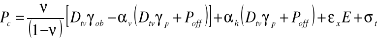
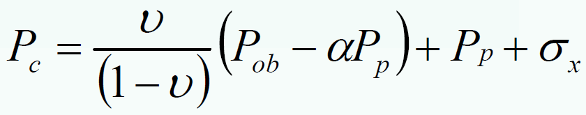
GOHFER’S Total Closure Stress Equation

Pc = closure pressure, kPa
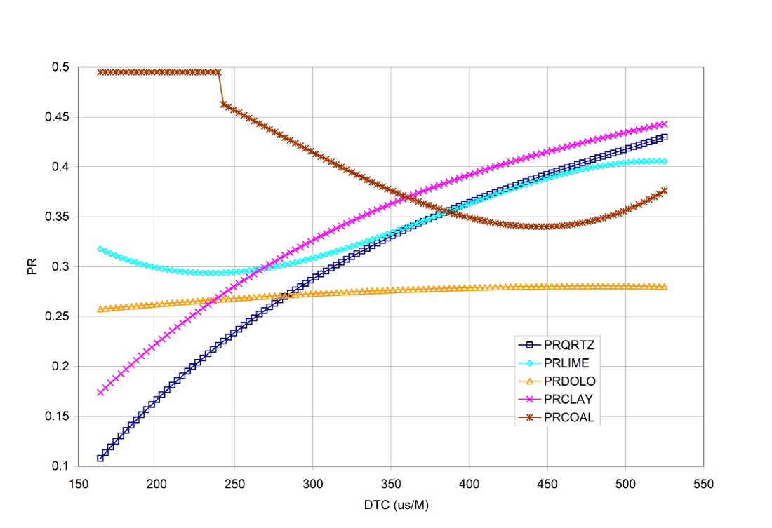
ν = Poisson’s Ratio
Dtv = true vertical depth, m
γob = overburden stress gradient, kPa/m
γp = pore fluid gradient, kPa/m
αv = vertical Biot’s poroelastic constant
αh = horizontal Biot’s poroelastic constant
Poff = pore pressure offset, kPa
εx = regional horizontal strain, microstrains
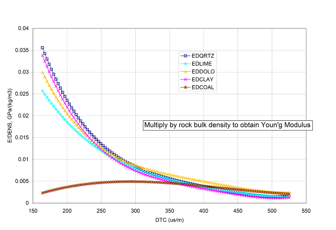
E = Young’s Modulus, GPa
σt = regional horizontal tectonic stress, kPa

• Closure stress is calculated using GOHFER’S Total Stress equation and must be calibrated to local field conditions with a strain or stress correction factor.
• In tectonically active areas, the closure stress calculated from logs will be too low and will need to be increased.
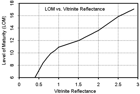
  • εx= regional horizontal strain
  • σt = regional horizontal tectonic stress
  • generally, the strain offset approach is favoured
• The best way to calibrate closure stress is to review fracturing work, or perform a minifrac.
• If possible, this step should be completed by the completion engineer (the person running the hydraulic frac simulation software).

Overburden Stress

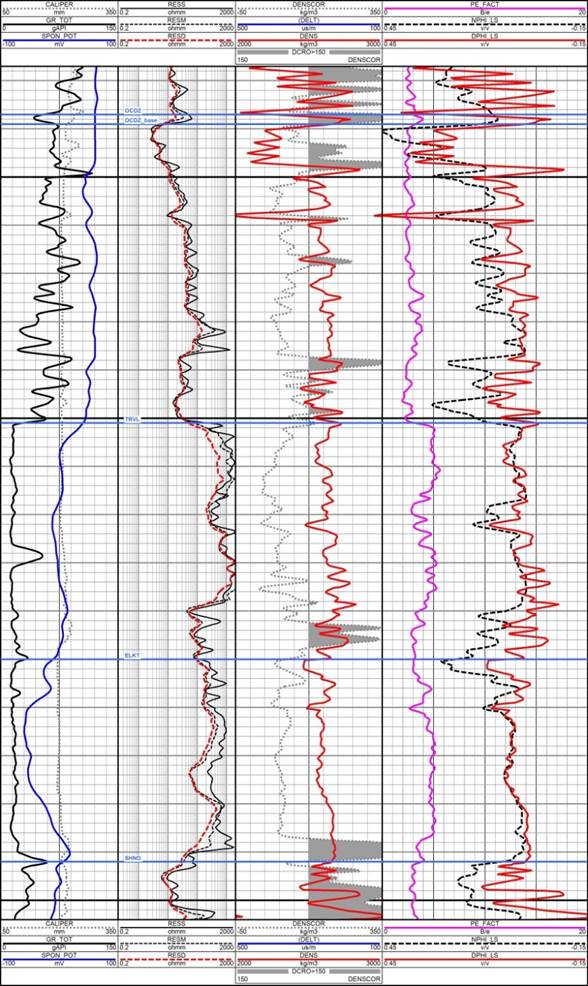
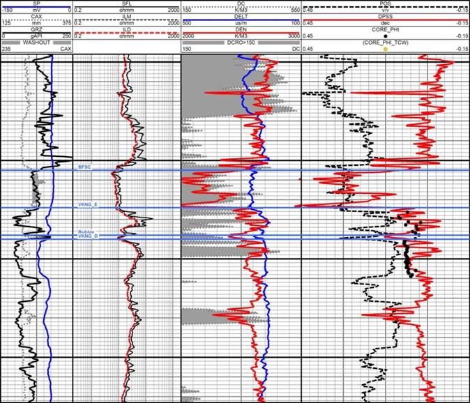
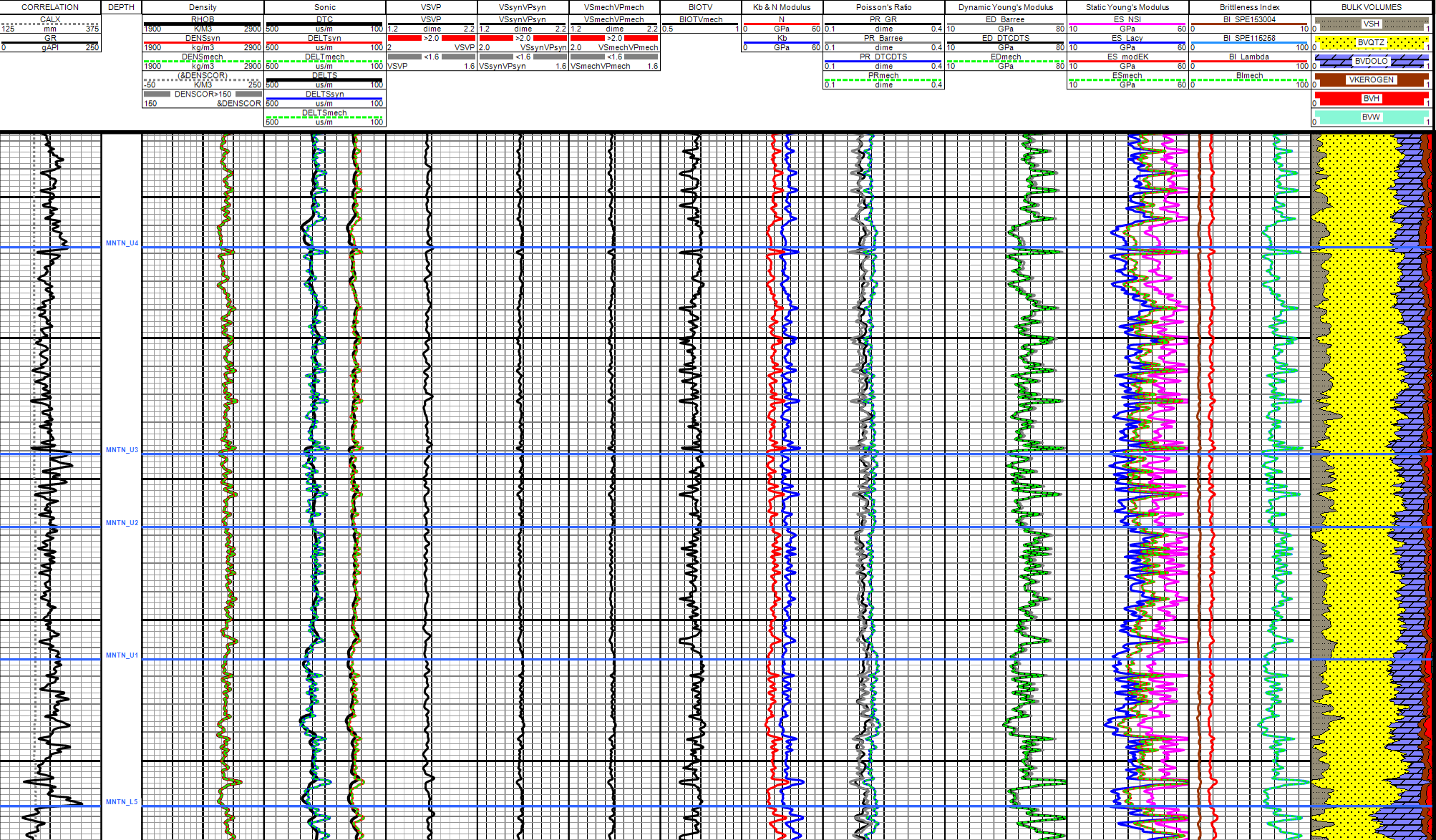
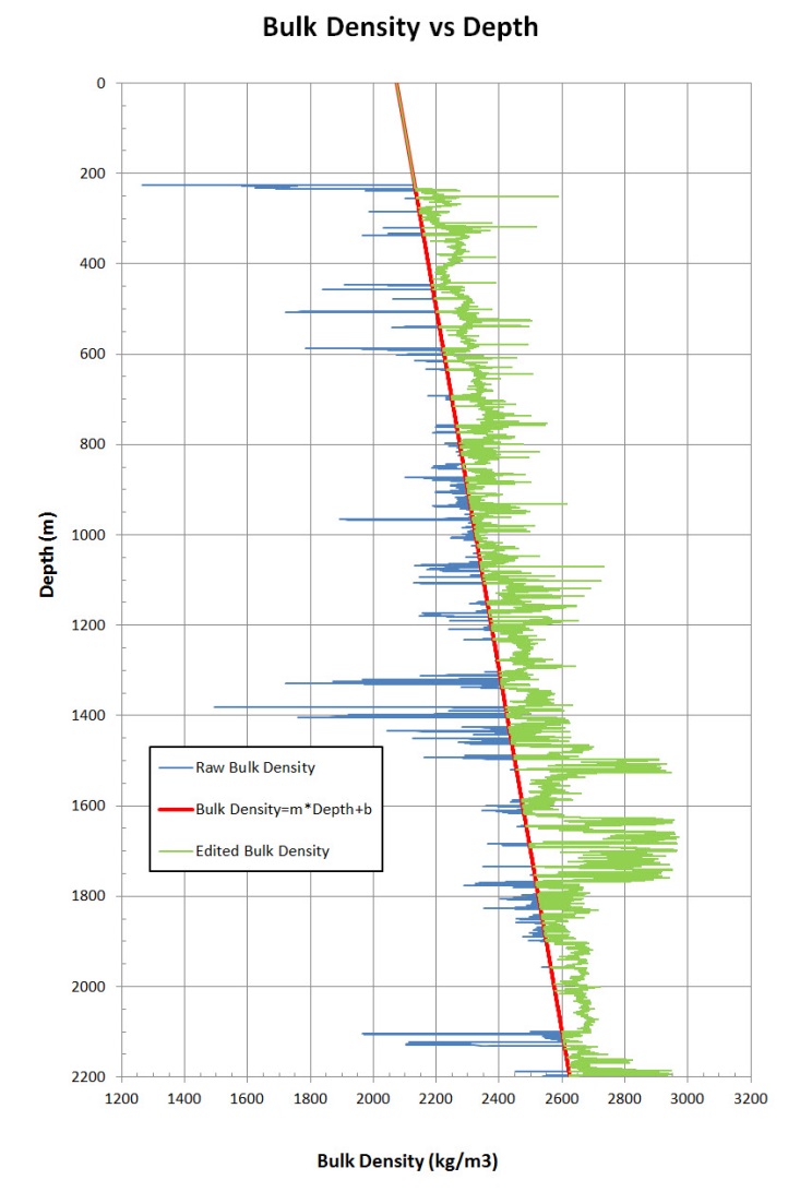
• The density log should be used to calculate overburden stress.
• Before the density log can be used, a synthetic log is created to remedy abnormally low data caused by bad hole, coal, etc.
  • Bad density data intervals are identified by running discriminators.
    • caliper and density correction logs are typically used
• The synthetic log is calibrated to intervals containing good quality density data and then integrated from treatment depth to shallowest log reading.
  • a bulk density value or density function must also be assigned from surface to shallowest log reading
• Overburden stress is an important input to the closure stress equation and will take some time and effort to calculate accurately

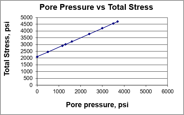
Pore Pressure (Barree & Associates)

• Field measured data should be used to assign pore pressure.
• Pore fluid supports part of the total stress.
• Pore pressure depletion increases net stress and leads to compaction.
• Pore pressure depletion decreases total (fracture closure) stress.

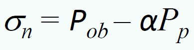
Biot’s Poroelastic Parameter (Barree & Associates)

• Barree defines Biot’s poroelastic constant as the efficiency with which internal pore pressure offsets the externally applied vertical total stress.
• As Biot decreases, net (intergranular) stress increases and pore pressure variations have less impact on net stress.

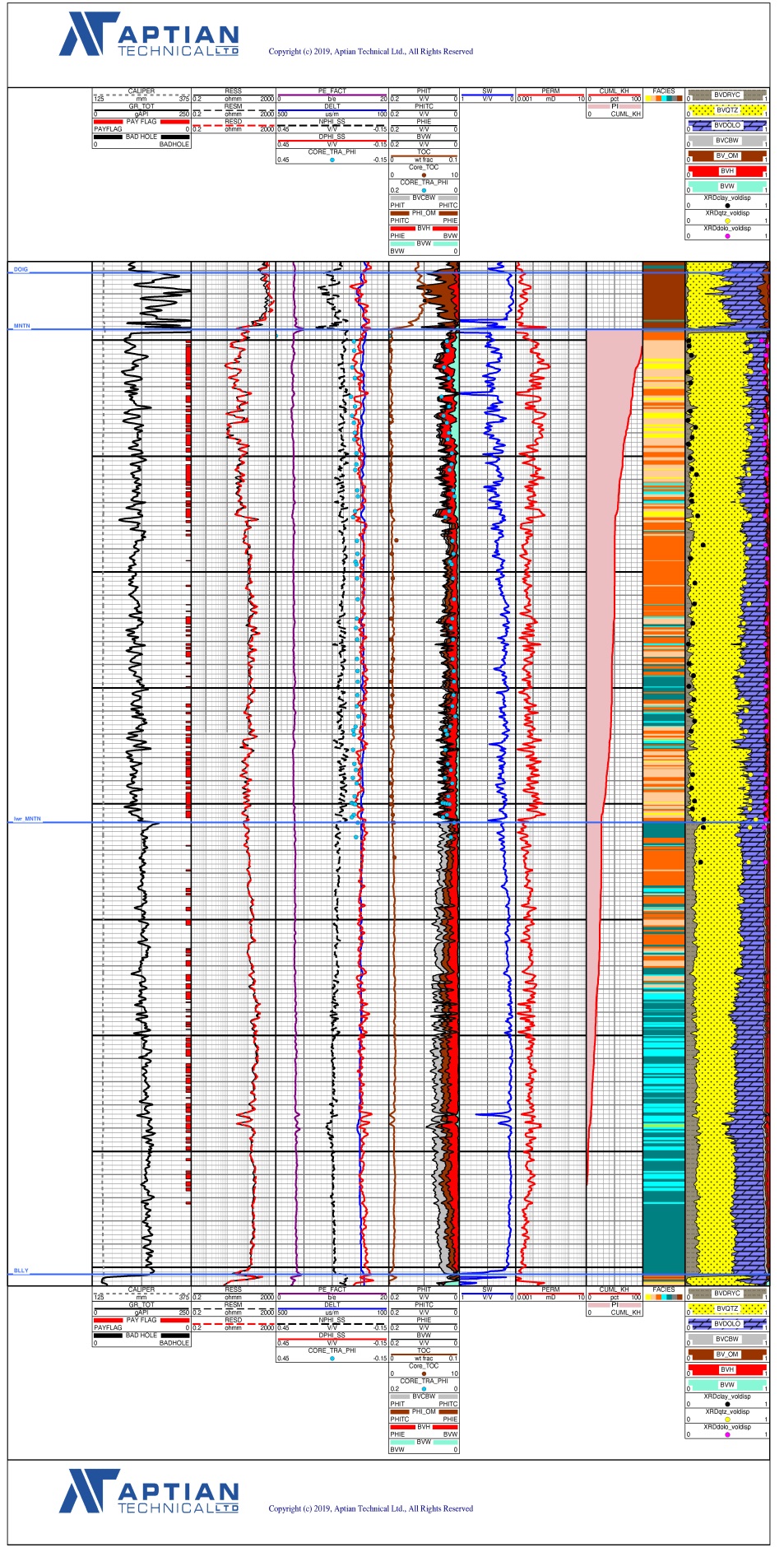
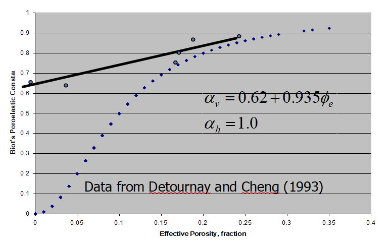
• Effective porosity from the quantitative analysis is used to calculate vertical Biot’s poroelastic parameter.
• Horizontal Biot’s poroelastic parameter is generally set equal to 1.

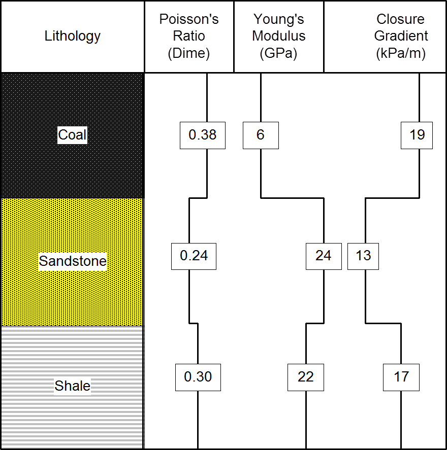
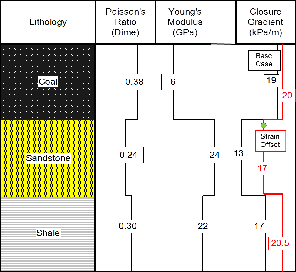
Closure stress base case

• no strain offset
• no stress offset

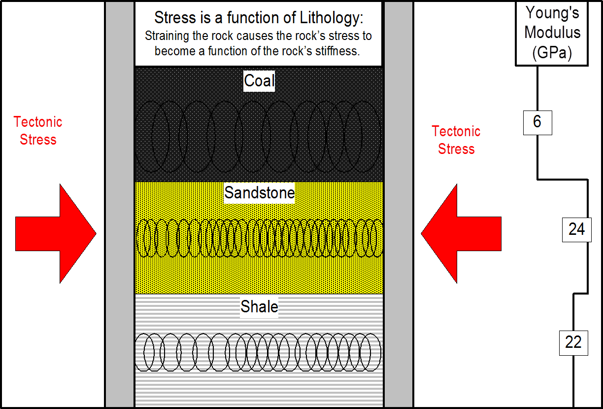
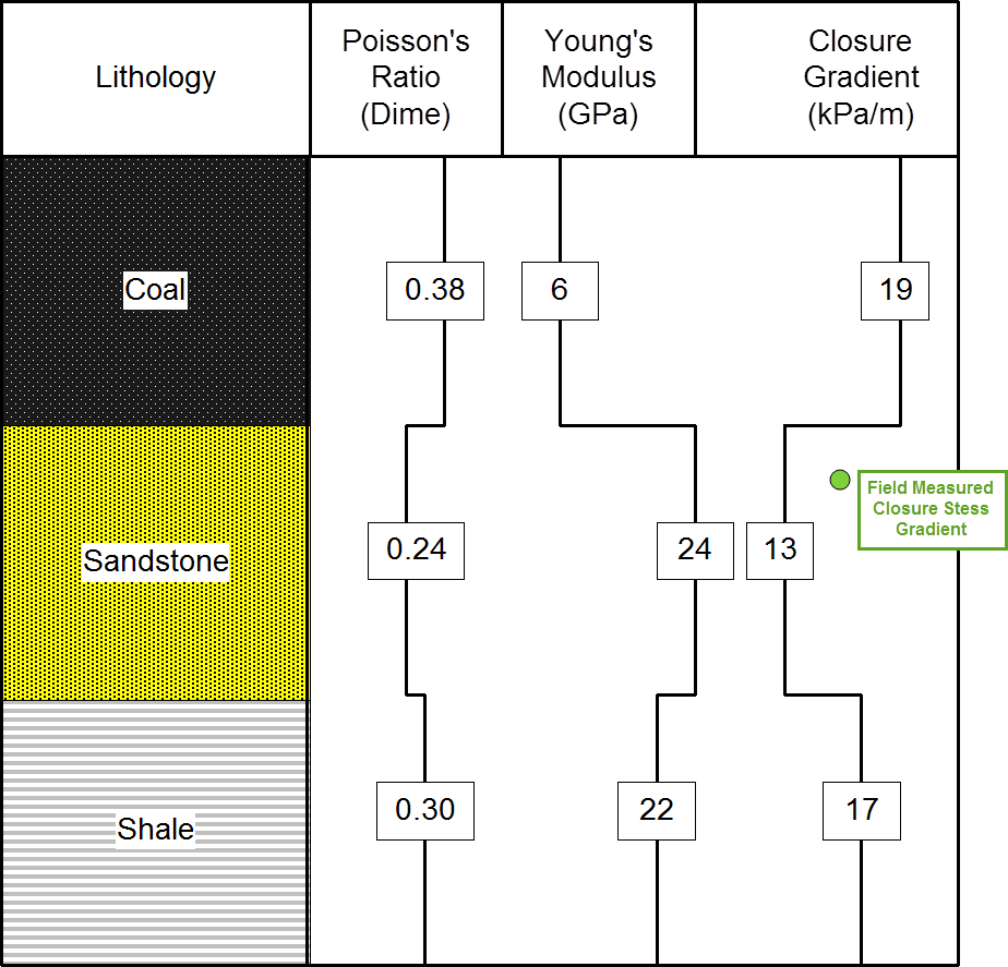
With Regional Tectonism Present

• With tectonism, the closure stress base case will not match field measured data.
  • a strain offset will need to be applied

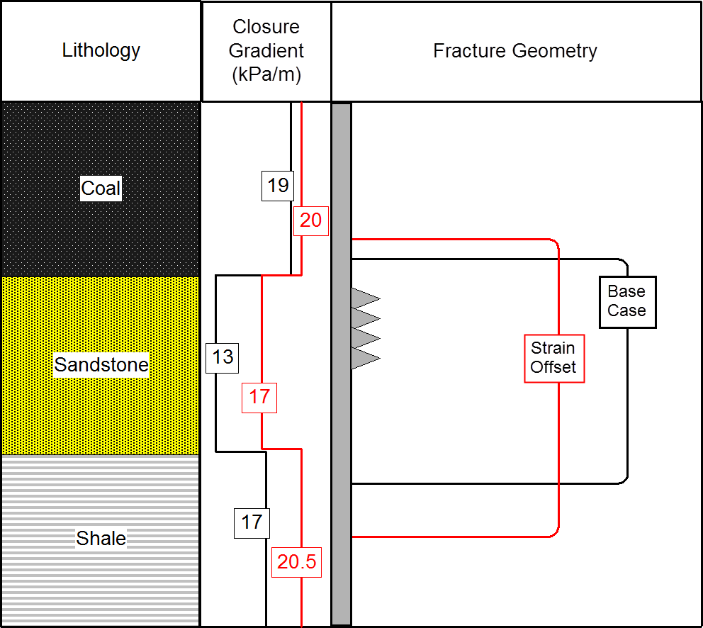
A match is achieved using a strain offset.

• Applying a strain offset can decrease the stress difference between the reservoir and non-reservoir intervals.
  • fracture geometry will be affected

Unconventional shale gas example

• Results from the custom calculation sequence match SCAL data very well.
• Next, results were used as input to reconstruct the density and sonic logs.
• The reconstructed logs were then used to calculate mechanical rock properties.

Clastic Example with Rough Bore Hole

• The reconstructed density and sonic logs were used to calculate mechanical rock properties.

• The twenty step petrophysical workflow has proven successful in many challenging reservoir environments, worldwide. To date, 300 projects for multiple clients have been completed. These projects comprise work on thousands of wells.
• A three well minimum is recommended for all projects.
  • Rarely will the subject well have all required data needed to complete a calibrated petrophysical analysis.
  • Offset wells should always be reviewed and used to put together the best data set possible.
  • The accuracy of the petrophysical model improves with an increased number of wells reviewed.
• Trying to perform a petrophysical analysis with hydraulic frac simulation software is not recommended.
  • Robust petrophysical software and an experienced petrophysicist are required to generate accurate mechanical rock properties.
• Closure stress calculation and calibration should, if possible, be carried out by an experienced completion engineer. This step should be run within the hydraulic frac simulation software.
  • field data must be reviewed and used for calibration
    • pore pressure
    • closure pressure
• Sufficient time and talent should be allowed by management for the process.
• The reconstruction step is particularly important for sonic and density logs.
  • small input errors amplify to become surprisingly large
  • Reconstructed logs should be used to calculate Young’s modulus and Poisson’s ratio.
    • essential input to stimulation design software packages
• A full suite of TOC and XRD mineralogy from samples, along with core porosity and saturation data, are needed to calibrate results from any petrophysical analysis of unconventional reservoirs.
  • bulk clay and TOC are the two critical lab measurements
• Without valid calibration data, petrophysical analysis will have possible error bars too large to allow meaningful financial decisions.
• This deterministic workflow allows all available empirical data to be used in a logical and consistent manner at each step to calibrate and refine results.
• Petrophysical analysis results travel well beyond the initial need to know porosity and water saturation.
  • oil and gas in place
  • reservoir stimulation
  • placement of horizontal wells
  • financial reports
• The cost of the full analysis and reconstruction is trivial compared to the cost of completion, or worse, an unsuccessful completion design.

• Barree, R.D., Gilbert, J.V. and Conway, M.W.”Stress and Rock Property Profiling for Unconventional Reservoir Stimulation,” paper SPE 118703 presented at the 2009 SPE Hydraulic Fracturing Technology Conference held in the Woodlands, Texas, USA, 19-21 January 2009.
• Crain, E.R., “Crain’s Petrophysical Handbook.”, at http://www.spec2000.net, Rocky Mountain House, Alberta, Canada, 2013.
• Crain, E.R., and Holgate, Dorian. “Synthetic Log Curves: An Essential Ingredient For Successful Stimulation Design.” CSPG Reservoir Volume 40, Issue 5, May 2013: 19-24.
• Crain, E.R., and Holgate, Dorian. “A 12 Step Program to Reduce Uncertainty in Kerogen-Rich Reservoirs: Part 1 – Getting the Right Porosity.” CSPG Reservoir Volume 41, Issue 3, March 2014: 19-23.
• Crain, E.R., and Holgate, Dorian. “A 12 Step Program to Reduce Uncertainty in Kerogen-Rich Reservoirs: Part 2 – Getting the Right Hydrocarbon Volume.” CSPG Reservoir Volume 41, Issue 4, April 2014: 34-38.
• Crain, E.R., and Holgate, Dorian. “Digital Log Data To Mechanical Rock Properties For Stimulation Design,” presented at the GeoConvention Conference held in Calgary, Alberta, Canada, 12-16 May 2014.
• Lacy, L.L., “Dynamic Rock Mechanics Testing for Optimized Fracture Designs,” paper SPE 38716.
• Leshchyshyn, T.H., et. al., “Using Empirically Developed Rock Tables to Predict and History Match Fracture Stimulations,” paper SPE 86989.
• Mullen, Mike., Roundtree, Russel., Barree, R.D., “A Composite Determination of Mechanical Rock Properties for Stimulation Design (What To Do When You Don’t Have a Sonic Log),” paper SPE 108139.
• Rickman, Rick., and Mullen, Mike., et. al., “A Practical Use of Shale Petrophysics for Stimulation Design Optimization: All Shale Plays Are Not Clones of the Barnett Shale,” paper SPE 115258.